
The aim of this activity is to acquire the numerical values of a hand drawn plot using pixel values of its digital image.
The first thing I did, with the help of my classmates, was to find an old journal with a graph that is not digitally printed. I would say this was the hardest part of the activity. After a lot of searching, we finally found the journal entitled “The microbiological assay of amino acids in some Philippine legumes” by Nieves Portugal-Dayrit from the CS library. I chose a hand-drawn graph, photocopied it and then scanned it. This is the scanned image:

Next, I opened the image in GIMP 2.8. The first thing I did was correct for rotations. To do this i selected a proper grid spacing by going to Image > Configure grid, and then showed the grid by going to View. Then I rotated the image using Tools > Transform Tools > Rotate to align the axes with the grid.
Now to relate image pixel location with the physical values in the plot, I first need to know how many pixels a single physical unit takes (pixels per unit). I moved the mouse over the tick marks of both the X and Y axis and noted the pixel locations xp and yp. I took the difference between pixel locations of adjacent tick marks, and took the average difference. The number of pixels a single physical unit takes can then be calculated by taking the average difference divided by the physical interval of the tick marks. For example, if the pixel locations for the tick marks in the X axis are x1, x2, x3 and the physical interval is 2.5 (as in the image), the pixels per unit, say pu, is then:

I also took note of the pixel locations of the origin x_0 and y_0. I found the p_u‘s to be 162.08 and 804.4 for the X and Y axes respectively. Since a single unit in the X axis spans 162.08 pixels, the physical value x = 1 must have an xp equal to x0 + 162.08. x = 2 must have an xp equal to x0 + 2(162.08) and so on:

Rearranging, we get:

The same also applies to values in the Y axis except the sign is changed because yp = 0 at the top of the image:

Knowing the last two equations, I can simply take pixel locations of points in the curve and convert them to physical values. Using the mouse, I took pixel locations of 25 points, converted the locations to physical values, and plotted the values in Excel.
Here is the result:
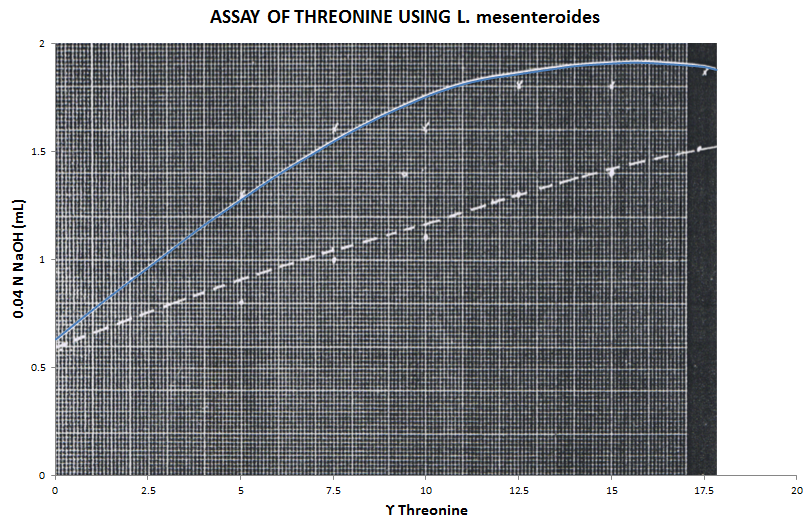
I used the image of the plot as a background of the Excel plot area. The reconstructed graph very closely replicates the scanned graph. Because of this, I would rate myself 9/10 for the reconstruction.

The limitation in the method I used is using the mouse to find pixel locations. That isn’t very accurate since the curve line has a width which contains a plural number of pixels. This resulted in very close but inexact values compared to the original plot.

John Kevin Sanchez and Jaime Olivares helped me in acquiring a photocopy of a hand-drawn graph.
References:
- M. Soriano, A2 – Digital Scanning, Applied Physics 186, National Institute of Physics, 2014.
- N. Portugal-Dayrit, “The microbiological assay of amino acids in some Philippine legumes,” College of Science, University of the Philippines Diliman, 1956.
Image references:
