Scilab Basics

In this activity, the aim is to create a number of synthetic images as a practice for future testing of algorithms or simulations of optical phenomena in imaging systems.

Sample code written in Scilab that creates a circular aperture was given to us. The code produces the image:

This was performed by first creating two 2D arrays (X and Y) containing x and y coordinates ranging from -1 to 1 using the ndgrid() function. The number of x and y elements are set using the variables nx and ny respectively.  With the line:

r = sqrt(X.^2 + Y.^2);

A matrix r is created that contains circle radius values. The value of r(x,y) is equal to the radius of a circle centered at (0,0) whose edge lies on (X(x,y),Y(x,y)). The matrix r represents the radius values of circles with varying sizes centered at the origin. When plotted, the matrix r looks like:

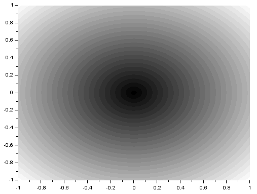
Then, a zero matrix A with the same size as r was created. With the line:

A (find(abs(r)<0.5) ) = 1;

Indices where r < 0.5 are chosen and the value of A at these indices is changed to 1. This will form a circle with a radius equal to the value in matrix r which is closest to but less than 0.5. For high nx and ny, this will produce a radius which is approximately 0.5.

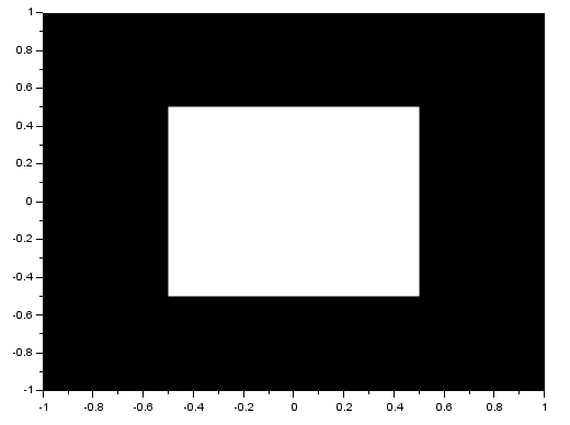
Other synthetic images can be made by varying A or r. To make a centered square aperture, I replaced last line above with:

A (find(abs(X)<0.5) ) = 1;
A (find(abs(Y)>0.5) ) = 0;

First, indices representing |x| < 0.5, the value of A is changed to 1. This will form a rectangle. The second line turns the image into a square by returning the values where |y| > 0.5 to 0. The resulting image is:

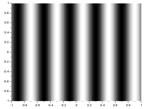
To produce a sinusoid along the x-direction or a corrugated roof, r was simply adjusted to:

r= sin(X*5*%pi);

and was plotted.  The resulting image is:

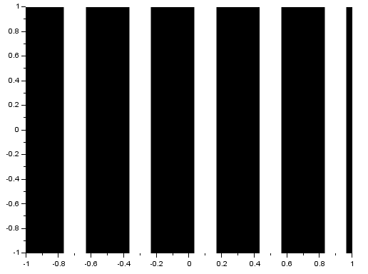
To produce grating along x, I simply added the line:

A (find(r>0.5) ) = 1;

to the code for the sinusoid. This is a discrete version of the sinusoid since certain values of r are changed to just either 1 or 0. The result is:

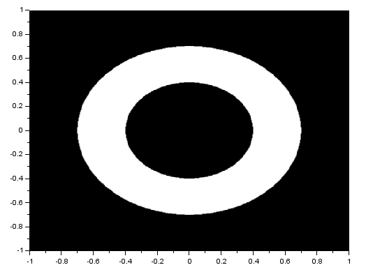
To produce an annulus, I simply adjusted the original code to produce two circles of different size. One circle made of 1 values and the other made of 0 values. The resulting image is:

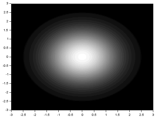
To create a circular aperture with Gaussian transparency, the range was changed to -3 to 3 and the matrix A in the original code was replaced with:

G = 1/sqrt(2*%pi)*exp(-(r.^2)/2);
G (find(r>2.5) ) = 0;

The first line is simply the equation for the Gaussian Distribution. The second line blackens the area outside of the circle with radius 0.8. The range was changed so that more shades of gray are used. The result is:

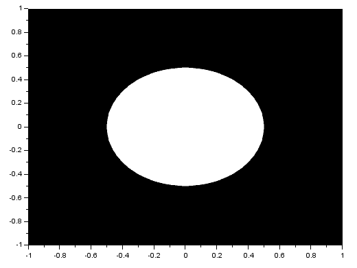
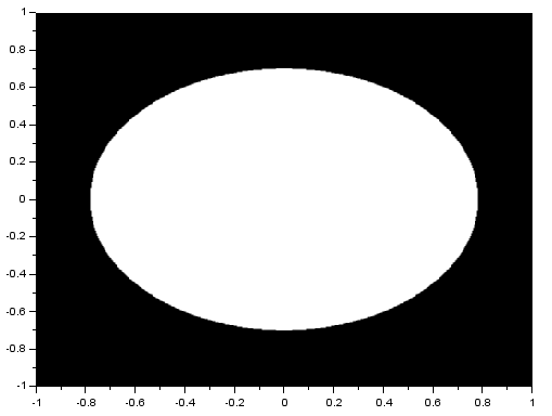
An ellipse can be made by simply multiplying either X or Y in the original code by a constant with a magnitude less than 1.  The result is:

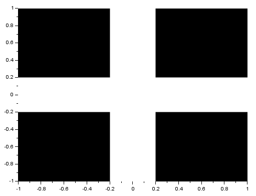
A cross can be made by adjusting the code for the square image. Replacing the lines assigning values to A with:

A (find(abs(X)<0.2) ) = 1;
A (find(abs(Y)<0.2) ) = 1;

forms the image:

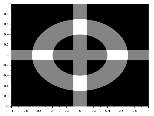
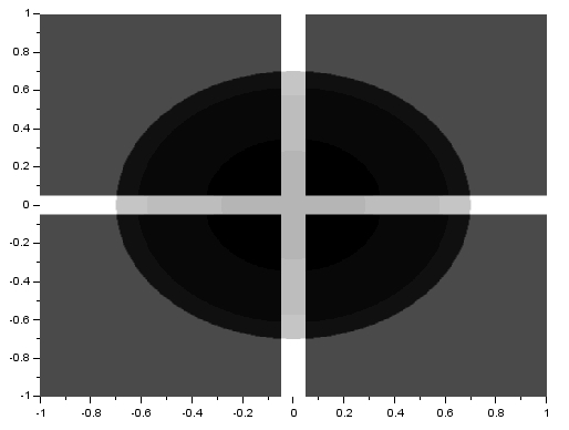
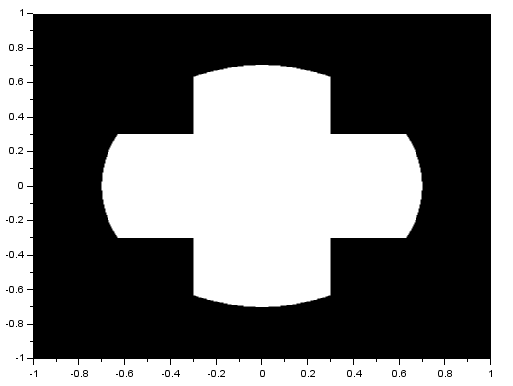
Using the matrix for the cross image and adding it to the annulus matrix, subtracting the gauss matrix from it, and multiplying it to the circle matrix, the following images were formed:

             

Figuring out how to produce each image was fun and maybe being new to programming in Scilab made it even more fun. Even figuring out some new functions like find() was enjoyable. Since I have produced all the required images and explored the outcomes of combining matrices for different images, i would rate myself with a grade of 10.

                                          *ten tententenen ten tenenenenen ten ten ten teneeen

References:

M. Soriano, “A3 – Scilab Basics,” Applied Physics 186, National Institute of Physics, 2014.

Image References:

http://cuddlychriscrymsyn.tumblr.com/

Digital Scanning

The aim of this activity is to acquire the numerical values of a hand drawn plot using pixel values of its digital image.

The first thing I did, with the help of my classmates, was to find an old journal with a graph that is not digitally printed. I would say this was the hardest part of the activity. After a lot of searching, we finally found the journal entitled “The microbiological assay of amino acids in some Philippine legumes” by Nieves Portugal-Dayrit from the CS library. I chose a hand-drawn graph, photocopied it and then scanned it. This is the scanned image:

Next, I opened the image in GIMP 2.8. The first thing I did was correct for  rotations. To do this i selected a proper grid spacing by going to Image > Configure grid, and then showed the grid by going to View. Then I rotated the image using Tools > Transform Tools > Rotate to align the axes with the grid.

Now to relate image pixel location with the physical values in the plot, I first need to know how many pixels a single physical unit takes (pixels per unit). I moved the mouse over the tick marks of both the X and Y axis and noted the pixel locations x_p and y_p. I took the difference between pixel locations of adjacent tick marks, and took the average difference. The number of pixels a single physical unit takes can then be calculated by taking the average difference divided by the physical interval of the tick marks. For example, if the pixel locations for the tick marks in the X axis are x₁, x₂, x₃ and the physical interval is 2.5 (as in the image), the pixels per unit, say p_u, is then:

I also took note of the pixel locations of the origin x_0 and y_0. I found the p_u‘s to be 162.08 and 804.4 for the X and Y axes respectively. Since a single unit in the X axis spans 162.08 pixels, the physical value x = 1 must have an x_p equal to x₀ + 162.08. x = 2 must have an x_p equal to x₀ + 2(162.08) and so on:

Rearranging, we get:

The same also applies to values in the Y axis except the sign is changed because y_p = 0 at the top of the image:

Knowing the last two equations, I can simply take pixel locations of points in the curve and convert them to physical values. Using the mouse, I took pixel locations of 25 points, converted the locations to physical values, and plotted the values in Excel.

Here is the result:

I used the image of the plot as a background of the Excel plot area. The reconstructed graph very closely replicates the scanned graph. Because of this, I would rate myself 9/10 for the reconstruction.

The limitation in the method I used is using the mouse to find pixel locations. That isn’t very accurate since the curve line has a width which contains a plural number of pixels. This resulted in very close but inexact values compared to the original plot.

John Kevin Sanchez and Jaime Olivares helped me in acquiring a photocopy of a hand-drawn graph.

References:

1. M. Soriano, A2 – Digital Scanning, Applied Physics 186, National Institute of Physics, 2014.
2. N. Portugal-Dayrit, “The microbiological assay of amino acids in some Philippine legumes,” College of Science, University of the Philippines Diliman, 1956.

Image references:

http://memegenerator.net