Image Segmentation

The aim in this activity is to segment images by picking a region of interest (ROI) and then processing the images based on features unique to the ROI.

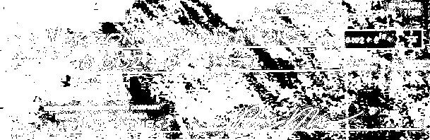
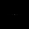
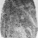
For grayscale images where the ROI has a distinct grayscale range, segmentation can easily be done by using thresholding. For example, lets take the image:

Using Scilab, the grayscale histogram of the image read as I can be computed and plotted using the lines [1]:

[count, cells] = imhist(I, 256);
plot (cells, count);

This results in:

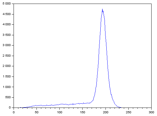
The large peak corresponds to the background pixels which are lighter than the text. To segment the text, we can assume that using a threshold of 125 can be used since it is less than and far from the pixel values of the peak. This can be implemented using the lines [1]:

threshold = 125;
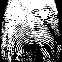
BW = I < threshold;

This results in:

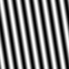
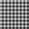
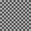
where only the pixels having values less than the threshold of 125 are colored white. Using threshold values of 50, 100, 150, and 200, (left to right, up to down) I got:

We can see that using a lower threshold than needed will segment fewer details while using a higher threshold than needed will include too much unwanted details in the segmented image.

The problem of segmentation for colored images is more complicated. ROI’s that have unique features in a colored image might not be distinct after converting the image to grayscale [1]. Also, when segmenting images that have 3D objects, the variation in shading must be considered. Because of this, it is better to represent colors using the normalized chromaticity coordinates or NCC [1].

The NCC can be computed using the equation:

where . Since b is dependent on r and g, the chromaticity can be represented by using just the two coordinates r and g. I represents the brightness information [1]. The normalized chromaticity space is then shown in the plot:

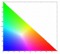
where the x-axis is r and the y-axis is g [1].

A. Parametric Estimation

Segmentation can be done by calculating the probability that a pixel belongs to the color distribution of the ROI. To do this, we can crop a subregion of the ROI and compute its histogram. When normalized by the number of pixels, the histogram is already the probability distribution function (PDF) of the color. Assuming a Gaussian distribution for r and g, independently, of the cropped region, the means , , and standard deviations ,  can be computed [1]. The probability is then computed using the equation:

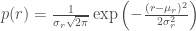
A similar equation can be used for p(g). The joint probability is then the product of p(r) and p(g) and can be plotted to produce a segmented image [1].

B. Non-Parametric Estimation

Histogram backprojection is a method where a pixel value in the image is given a value equal to its histogram value in the normalized chromaticity space. This can be used to segment images by manually looking up the histogram values. A 2D Histogram can be obtained by converting the r and g values to integers and binning the image values to a matrix. This can be implemented using the code [1]:

BINS = 180;
rint = round (r*(BINS-1) + 1);
gint = round (g*(BINS-1) + 1);
colors = gint(:) + (rint(:)-1)*BINS;
hist = zeros(BINS,BINS);
for row = 1:BINS
for col = 1:(BINS-row+1)
hist(row,col) = length( find(colors==( ((col + (row-1)*BINS)))));
end;
end;

where r and g are taken from the ROI. Then, the segmented image can be computed using the code [1]:

rint = round (r*(BINS-1) + 1);
gint = round (g*(BINS-1) + 1);
[x, y] = size(sub);
result = zeros(x, y);
for i = 1:x
for j = 1:y
result(i,j) = hist(rint(i,j), gint(i,j));
end;
end;

where r and g are taken from the subject image.

C. Results

The first image I segmented is a drawing of one of my favorite monsters from the game Monster Rancher, Mocchi:

souce: deviantart

The colors found on its head (green), lips (yellow), body (cream), and belly (cream) all appear solid. I cropped the following ROIs:

                  

for the four parts. After applying parametric estimation, I got (left to right, up to down):

We can see that the corresponding body parts of Mocchi, depending on the cropped ROI, were successfully segmented. After looking closely at the image, I saw that there are actually distortions near the black pixels (Mocchi’s edges). These distortions are the reason why the segmented images do not exactly follow Mocchi’s shape.

Next, I segmented an image of pick-up sticks:

source: choicesdomatter.org

First, I used an ROI from a green stick that has minimal shading variations:

Using parametric estimation, I got the following segmented image:

We can see that some areas are not segmented perfectly. These areas are those of really bright or really dark shading. Using an ROI from a stick with more shading variations:

I got:

We can see that the green sticks are clearly identified by the white pixels, however, other areas are no longer black. This is because the features of the new ROI are no longer unique to just the green sticks. For the other colors, I will continue with using ROIs taken from sticks with minimal shading variations:

                 

I will also apply non-parametric estimation. First, I plotted the histogram of the ROIs, respectively:

If we look at the plot of the normalized chromaticity space again, we can see that the location of the peaks are located inside the corresponding expected regions. Therefore we can say that the histograms are correct. For the green, red, yellow, and blue ROIs, respectively, I got a segmented image using parametric estimation (left) and non-parametric (right) estimation:

green:

red:

yellow:

blue:

We can see that using parametric estimation segments the corresponding pick-up sticks more accurately than using non-parametric estimation. For this case, using non-parametric estimation identifies fewer pixels to be similar to the ROI since it directly uses the histogram instead of using a probability distribution. Therefore it is not suitable for use when segmenting images with objects that have really small widths such as these pick-up sticks. After using non-parametric estimation on the image of Mocchi using the same ROIs shown in the first part of the results, I got:

We can see that the segmentation is still successful since the parts corresponding to the different ROIs are large enough.

This activity was fun because I can instantly be gratified by the results since they can be confirmed by just looking at the segmented images.

Since I was able to obtain all the required images, I will rate myself with 10/10. Also, thanks to John Kevin Sanchez, Ralph Aguinaldo, and Gio Jubilo for helping me in correcting my equations and understanding backprojection.

References:

1. M. Soriano, “A7 – Image Segmentation,” Applied Physics 186, National Institute of Physics, 2014.

Image Reference:

img-comment-fun

Properties and Applications of the 2D Fourier Transform

The aim in this activity is to investigate some more properties of the 2D Fourier Transform (FT) and to apply these properties in enhancing images.

A. Anamorphic property of FT of different 2D patterns

As we know, the FT space is in inverse dimension. Because of this, performing the FT on an image with an object that is wide in one axis will result in a narrow pattern in the spatial frequency axis [1]. As examples, I will show the FTs of different patterns. I implemented the FT in Scilab using the functions given in (Fourier Transform Model of Image Formation). For a tall rectangular aperture:

              

The FT is the image in the right. For a wide rectangular aperture:

               

We can see that the resulting rectangles in the y-axis for the wide rectangle are narrower than that of the tall rectangle. On the x-axis, we can see that the resulting rectangles are shorter for the tall rectangle. For two dots along the x-axis:

               

For two dots with a different separation distance:

               

We can see that the wider the space between the two dots is, the narrower the space between the peaks of the resulting sinusoid pattern (also, the higher the frequency).

B. Rotation Property of the Fourier Transform

Next, I will investigate the rotation property of the 2D FT where rotating a sinusoid results in a rotated FT [1]. The following images are of sinusoids and their resulting FTs:

The generated matrices used for these images have negative values. Since digital images have no negative values, these sinusoids are not perfect. Because of this, we see multiple dots in the FTs although they were expected to have only two dots which identify the sinusoids’ frequency. Still, we can observe the anamorphic property of the FT. We can see that the resulting dots farther from the center are produced for sinusoids which have closer peaks. To correct the sinusoids, I applied a constant bias so that all values are positive. I got the resulting sinusoid and its FT:

           

Now we can see fewer dots. The central dot comes from the applied bias. Given a signal or pattern, we can measure its actual frequency by performing the FT and measuring the distance of the two dots from the center. After applying a non-constant bias (a very low frequency sinusoid) to the sinusoid, I got:

           

If we look closely, we can see two dots near the central dot. These dots represent the frequency of the non-constant bias. If it is known that the bias has a very low frequency, the frequency of the signal can still be measured using its FT.

After rotating the sinusoid, I got:

           

We can see that the resulting FT pattern rotated as well. Then, I created a pattern formed by adding a sinusoid along the x-axis and a sinusoid along the y-axis. Both sinusoids have the same frequency. I got:

           

As expected, there are four dots in the resulting FT pattern. Two dots placed on the x-axis and two dots placed on the y-axis. When i multilpy the two sinusoids instead, I get:

           

The product of two sinusoids along the same axis is given by the following equation [2]:

We can see that the product is equivalent to the difference of two sinusoids with frequencies formed from the difference and sum of the frequencies of the original sinusoids. This adding and subtracting of frequencies could be the reason for the position of the dots in the resulting FT.

Finally, I added multiple rotated sinusoids to the previous pattern and performed the FT. I got:

          

Looking closely, we can see dots around the central dot and they actually form a circle. These dots represent the frequency of the 10 rotated sinusoids that I used. This further proves that a rotated sinusoid also has a rotated FT.

C. Convolution Theorem Redux

I performed the FT on an image with two circles along the x-axis:

           

We know that the FT of two dots is a sinusoid and that the FT of a circle is composed of rings. Noting that, we see that the resulting FT here resembles the product of the FT of two dots and the FT of a circle. I also performed the FT on an image with two squares and got:

           

Again, the resulting FT looks like the product of the FT of two dots and the FT of a square. Using two Gaussians of different , I got:

We recall that the FT of a Gaussian is also a Gaussian. Again, the resulting FT looks like the product of the FT of two dots and the FT of a square. From the three previous results, we can observe that the inverse FT of the product of the FT of two dots and the FT of another pattern results in a replication of the pattern at the position of the dots. This, in fact, demonstrates the convolution theorem [1]:

A dot in a 2D image actually represents a dirac delta function. We know that the convolution of a dirac delta and a function f(t) replicates f(t) in the location of the dirac delta. Knowing this, we can apply it using an image containing dots and an image containing a distinct pattern. I convoluted a 3×3 pattern which forms a cross (x) with the following image:

and got:

We can see that if we invert x and y in the resulting image, the cross pattern will appear at the location of the points. The axes were inverted because quadrants are shifted when using the fft2() function in Scilab.

Next, I performed the FT on equally spaced dots, with a different spacing for each image:

The second batch of images are the resulting FTs for each corresponding image. For each FT, the sinusoids produced by the multiple dots must have accumulated to form dots with a different spacing. Again, we can observe the anamorphic property of the FT. Knowing the appearance of the FT’s of different patterns, such as this, can be used in constructing filters for image enhancement.

D. Fingerprint: Ridge Enhancement

Next, lets apply the convolution theorem to enhance images. I took an image of my fingerprint, turned it to grayscale, and binarized it.

We can see that there are some areas with blotches and light areas. I took the FT of the grayscale image and got:

We can see that there is a distinct ring. This ring must represent the frequencies of the ridges of my fingerprint. Knowing this, I constructed the filter:

I multiplied this filter with the FT and performed an inverse FT. I got the resulting enhanced fingerprint and binarized it using the same threshold.

           

We can see that the ridges are now more distinct and the blotches have been reduced.

E. Lunar Landing Scanned Pictures: Line removal

I applied the same method to the image:

We can see that there are vertical lines throughout the image. It’s not obvious but there are also horizontal lines. I took its FT and got:

Looking closely we can see that there are several dots along the x and y axes. These must represent the frequencies of the vertical and horizontal lines. I constructed the following filter:

After doing the same thing as in part D, but instead on the RGB components, individually, and then forming the colored image again, I got:

We can see that the vertical and horizontal lines have been removed.

F. Canvas Weave Modeling and Removal

For a final application, let’s look at the image:

We can see the weave patterns of the canvas. I performed the FT on the image and got:

We can see some dots along the x and y axes and four more dots that form the corners of a rectangle. These dots must represent the frequencies of the weave patterns. I then constructed the filter:

After applying the same method as in part E, I got:

We can see that the presence of the weave patterns has been significantly reduced. To check the filter I used, I took the inverse FT of the filter’s inverse and got:

We can see that it resembles the weave pattern in the painting. Using the convolution theorem by multiplying the inverse of the FT of the pattern we want removed (the filter) with the FT of the image, and then taking the inverse FT is an easy way of enhancing images.

This activity was very long but was very fun to do especially when I actually tried to enhance images. Although there are many more applications in using the FT, I feel like this is some sort of culmination of all the practice done in the previous activity and even of the required study we did on the Fourier Transform in our math and physics subjects. Since I was able to produce all the required images, I will rate myself with 10/10.

References:

1. M. Soriano, “A6 – Properties and Applications of the 2D
   Fourier Transform,” Applied Physics 186, National Institute of Physics, 2014.
2. ” Table of Trigonometric Identities,” S.O.S Mathematics, 2015. Retrieved from: http://www.sosmath.com/trig/Trig5/tritacg5/trig5.html

Image Reference:

http://mrwgifs.com/squall-rinoa-zell-victory-poses-in-final-fantasy-8/