
The aim in this activity is to familiarize with the use of the Fourier Transform to form images and some of its simple applications like template matching and edge detection.
The Fourier Transform
The Fourier Transform or FT is a linear transform that converts a signal that has dimensions of space into a signal in inverse space or spatial frequency. The FT of an image f(x,y) is given by the equation

where 

The Fast Fourier Transform of FFT is an efficient implementation of the FT made by Cooley and Turkey. In Scilab, the FFT routine is called using the function fft2() for 2D signals [1].
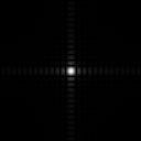
I created an image of a circle:

In Scilab, I read the image using imread() and converted it to grayscale using mat2gray(). I performed the FT on the matrix using fft2() and got the resulting image:

The quadrants of this image still need to be shifted because the output of fft2() has interchanged quadrants [1]. After using fftshift(), I got the resulting image:
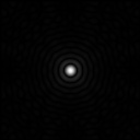

The image in the right is just a zoomed image. The resulting frequency pattern is formed of a small circle and concentric rings. This was the expected result for a circle image. If we consider the circle to be in the frequency domain, two points that have the same distance from the center will have an inverse FT that will be a sinusoid with a frequency given by the distance. Since the circle is made of many points with equal distance from the center, it will form multiple sinusoids with different orientations that will ultimately form concentric rings.
After applying fft2() twice on the image, i got the resulting image:

This is just similar to the original image but just slightly shifted. This is the result since applying the fft2() twice will just invert the image back to its original dimensions. If I take the real and imaginary parts, respectively, of the FT of the circle image, I get:


confirming that the FT is complex. I also created an image of the letter A:

After taking the FFT, shifted FFT, and applying the FFT twice, respectively, I got:
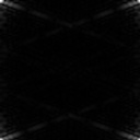
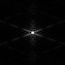

In the shifted FFT, the cross comes from the sides of the letter A and the vertical pattern in the center comes from the horizontal line of the letter A and its top. We can see that after applying the FFT twice, the resulting image is similar to the original. This time it is inverted because of the interchanged quadrants. Taking the real and imaginary parts of the image’s FT, I got:


FTs of Different Images
Next I will show images and their corresponding shifted FFTs. First for a sinusoid along x:

For this image, I first shifted the pixel values so that they are all positive. The resulting FT image is formed of 3 dots. The central dot is there because of the shifting of the image. This is similar to what happens when taking the FT of a voltage signal with an offset to have only positive values. The other dots represent the frequency of the sinusoid.
Then, for a double slit:


The left most image is just a zoomed image. Using the FT on the double slit simulates Young’s experiment that results in a diffraction pattern made of fringes when letting light pass through two apertures or slits.
Next, for an image of a square:
The resulting image is formed of a small square at the center and small rectangles formed on its sides. If I use a smaller square, I get:

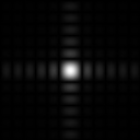
We can see that the resulting frequency pattern became larger. This is because after applying the FT, small features become big and large features become small [2].
Lastly, for a 2D Gaussian bell curve:


The resulting FT is also a Gaussian curve. Like the square image, using a smaller Gaussian curve as the image will yield a larger FT.
Convolution and Simulation of an Imaging Device
Next I perform a convolution which is similar to a smearing of one function with another [1]. The convolution between two 2D functions f and g is given by:

The resulting function h will have properties taken from the two functions f and g. For an imaging system, the f can represent the object, g can represent the transfer function (e.g. finite size of lens), and h can represent the produced image [1]. Linear transformations obey the convolution theorem [1]:

meaning i can compute the result h by taking the inverse of the product of Fourier Transforms H.
I performed a convolution between an image of the letters “VIP” and an image of a circle:


I first took the FFT of the vip image and multiplied it to the matrix of the circle image since it is already in the Fourier plane [1]. Then I took the inverse FFT of the resulting product. For circles of radius 0.2, 0.4, 0.6, and 0.8, respectively, I got:


We can see that the resulting image becomes clearer as the radius of the circle is increased. This is a simulation of an imaging device where the circle represents the aperture. As expected, using a larger aperture results in a clearer image.
Correlation and Template Matching
The correlation between two 2-D functions f and g is given by the equation:

where the correlation p measures the degree of similarity between the two functions. It can also be calculated using the equation:

where P, F, and G are the FTs of p, f, and g and the asterisk stands for complex conjugation.
I took the correlation between the two images:


This was done by taking the product of the FT of the A image and the conjugate of the FT of the text image. The correlation image is then the inverse FFT of the product. The resulting output is:

We can see that only the parts where there is a letter A in the text image are clear while the other parts are blurry and unreadable.
Edge Detection
Edge detection was performed by convolving the VIP image with a 3×3 matrix pattern of an edge that has a total sum of zero. For example, a horizontal edge can be represented by the matrix [1]:
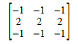
Convolving this with the VIP image resulted with the output:

We can see that the horizontal edges of the letters are more visible than the other parts of the letters. Using other edge patterns such as a vertical, diagonal, and spot pattern, respectively, resulted with:


We can see that depending on the edge pattern used, the edges with the same orientation with the pattern become more visible. Using a spot pattern, the edges of the letters on all orientations were detected.
This activity was fun because we had to generate a lot of images. Interestingly, the harder part of the activity for me was controlling the format of the images such as using mat2gray() on the output rather than the part where I apply the Fourer Transform or perform a convolution. With this problem I got some help from my classmates Martin Francis D. Bartolome and John Kevin Sanchez. Since I was able to generate all the required images, I will rate myself with 10/10.
References:
- M. Soriano, “A5 – Fourier Transform Model of Image
Formation, ” Applied Physics 186, National Institute of Physics, 2014. - F. Weinhaus, “ImageMagick v6 Examples — Fourier Transforms”, imagemagick.org, 2011. Retrieved from: http://www.imagemagick.org/Usage/fourier/
- P. J. Bevel, “The Fourier Transform at Work: Young’s Experiment,” The Fourier Transform .com, 2010. Retrieved from: http://www.thefouriertransform.com/applications/diffraction3.php
